Modelling a gallium arsenide surface

This example shows how to use the atomistic simulation environment or ASE for short, to set up and run a particular calculation of a gallium arsenide surface. ASE is a Python package to simplify the process of setting up, running and analysing results from atomistic simulations across different simulation codes. For more details on the integration DFTK provides with ASE, see Atomistic simulation environment (ASE).

In this example we will consider modelling the (1, 1, 0) GaAs surface separated by vacuum.

Parameters of the calculation. Since this surface is far from easy to converge, we made the problem simpler by choosing a smaller Ecut and smaller values for n_GaAs and n_vacuum. More interesting settings are Ecut = 15 and n_GaAs = n_vacuum = 20.

miller = (1, 1, 0)   # Surface Miller indices
n_GaAs = 2           # Number of GaAs layers
n_vacuum = 4         # Number of vacuum layers
Ecut = 5             # Hartree
kgrid = (4, 4, 1);   # Monkhorst-Pack mesh

Use ASE to build the structure:

using ASEconvert
using PythonCall

a = 5.6537  # GaAs lattice parameter in Ångström (because ASE uses Å as length unit)
gaas = ase.build.bulk("GaAs", "zincblende"; a)
surface = ase.build.surface(gaas, miller, n_GaAs, 0, periodic=true);

Get the amount of vacuum in Ångström we need to add

d_vacuum = maximum(maximum, surface.cell) / n_GaAs * n_vacuum
surface = ase.build.surface(gaas, miller, n_GaAs, d_vacuum, periodic=true);

Write an image of the surface and embed it as a nice illustration:

ase.io.write("surface.png", surface * pytuple((3, 3, 1)), rotation="-90x, 30y, -75z")

Python: None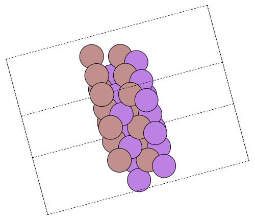

Use the pyconvert function from PythonCall to convert the ASE atoms to an AtomsBase-compatible system. This can then be used in the same way as other AtomsBase systems (see AtomsBase integration for details) to construct a DFTK model:

using DFTK
using PseudoPotentialData

pseudopotentials = PseudoFamily("cp2k.nc.sr.pbe.v0_1.largecore.gth")
model = model_DFT(pyconvert(AbstractSystem, surface);
                  functionals=PBE(),
                  temperature=1e-3,
                  smearing=DFTK.Smearing.Gaussian(),
                  pseudopotentials)

Model(gga_x_pbe+gga_c_pbe, 3D):
    lattice (in Bohr)    : [7.55469   , 0         , 0         ]
                           [0         , 7.55469   , 0         ]
                           [0         , 0         , 40.0648   ]
    unit cell volume     : 2286.6 Bohr³

    atoms                : As₂Ga₂
    pseudopot. family    : PseudoFamily("cp2k.nc.sr.pbe.v0_1.largecore.gth")

    num. electrons       : 16
    spin polarization    : none
    temperature          : 0.001 Ha
    smearing             : DFTK.Smearing.Gaussian()

    terms                : Kinetic()
                           AtomicLocal()
                           AtomicNonlocal()
                           Ewald(nothing)
                           PspCorrection()
                           Hartree()
                           Xc(gga_x_pbe, gga_c_pbe)
                           Entropy()

In the above we use the pseudopotential keyword argument to assign the respective pseudopotentials to the imported model.atoms. Try lowering the SCF convergence tolerance (tol) or try mixing=KerkerMixing() to see the full challenge of this system.

basis  = PlaneWaveBasis(model; Ecut, kgrid)
scfres = self_consistent_field(basis; tol=1e-6, mixing=LdosMixing());

n     Energy            log10(ΔE)   log10(Δρ)   Diag   Δtime
---   ---------------   ---------   ---------   ----   ------
  1   -16.58920088376                   -0.58    5.2    487ms
  2   -16.72516486573       -0.87       -1.01    1.0    257ms
  3   -16.73055393540       -2.27       -1.57    2.2    405ms
  4   -16.73122373751       -3.17       -2.16    1.0    1.55s
  5   -16.73132264669       -4.00       -2.58    1.8    247ms
  6   -16.73133028617       -5.12       -2.83    1.9    253ms
  7   -16.73068262363   +   -3.19       -2.40    2.4    283ms
  8   -16.73130501737       -3.21       -2.87    2.4    265ms
  9   -16.73121803573   +   -4.06       -2.75    2.0    257ms
 10   -16.73133256930       -3.94       -3.32    1.6    227ms
 11   -16.73133938109       -5.17       -3.70    1.1    214ms
 12   -16.73133998227       -6.22       -3.90    1.6    245ms
 13   -16.73134017769       -6.71       -4.23    1.8    241ms
 14   -16.73134016644   +   -7.95       -4.50    1.8    261ms
 15   -16.73134019943       -7.48       -4.93    1.8    240ms
 16   -16.73134019939   +  -10.33       -5.21    1.7    251ms
 17   -16.73134019964       -9.60       -5.28    1.9    256ms
 18   -16.73134020042       -9.11       -5.90    1.0    208ms
 19   -16.73134020042   +  -13.75       -6.13    1.8    241ms

scfres.energies

Energy breakdown (in Ha):
    Kinetic             5.8593967 
    AtomicLocal         -105.6100030
    AtomicNonlocal      2.3494809 
    Ewald               35.5044300
    PspCorrection       0.2016043 
    Hartree             49.5614177
    Xc                  -4.5976634
    Entropy             -0.0000035

    total               -16.731340200419